Tutorial: GABLS1 LES Intercomparison Study for Stable Boundary Layers

Last updated: May 2026

This tutorial walks through a complete JAX-ALFA simulation from scratch using the GABLS1 LES intercomparison study as the working example. By the end you will have:

1. Created a run directory with a Config.py, initial-condition files, and a surface boundary-condition file.

2. Launched the solver and understood the log output.

3. Loaded the statistics output and produced the standard mean-profile plots.

References:

Beare, R. J., and Coauthors. (2006). An intercomparison of large-eddy simulations of the stable boundary layer. Boundary-Layer Meteorology, 118, 247–272.

Basu, S. and Porté-Agel, F. (2006). Large-eddy simulation of stably stratified atmospheric boundary layer turbulence: A scale-dependent dynamic modeling approach. Journal of the Atmospheric Sciences, 63, 2074–2091.

Dai, Y., Basu, S., Maronga, B., and de Roode, S. R. (2020). Addressing the grid-size sensitivity issue in large-eddy simulations of stable boundary layers. Boundary-Layer Meteorology, 178, 63–89.

SGS model used here: Locally Averaged Scale-Dependent Dynamic (LASDD) – Smagorinsky (optSgs = 1).

---

1. Case Overview

The GABLS1 case simulates a stable nocturnal boundary layer driven by a prescribed surface cooling rate. It is widely used as a reference benchmark because the forcing is simple, the quasi-steady state is reached within 9 h, and a large ensemble of LES results is available in the literature.

Parameter	Value
Domain	400 m × 400 m × 400 m
Grid	128 × 128 × 128
Grid spacing	≈ 3.15 m (isotropic)
Geostrophic wind	\(U_g = 8\) m s\(^{-1}\), \(V_g = 0\)
Coriolis parameter	\(f = 1.39 \times 10^{-4}\) s\(^{-1}\) (73° N)
Roughness lengths	\(z_{0m} = z_{0T} = 0.1\) m
Initial surface temperature	265 K
Surface cooling rate	0.25 K hr\(^{-1}\)
Simulation duration	9 h
Time step	0.1 s
SGS model	LASDD-SM (optSgs = 1)
Precision	double (use_double_precision = True)
Averaging window	hours 8–9 (quasi-steady state)

---

2. Prerequisites

Before running this tutorial, ensure JAX-ALFA and its dependencies are installed. See the Installation page for step-by-step instructions.

---

3. Directory Layout

A JAX-ALFA run lives in its own directory. The packaged GABLS1 reference run used in this tutorial has the structure below:

examples/SBL_GABLS1/runs/128x128x128_LASDD_SM_DP/
├── Config.py
├── CreateInputs_SBL_GABLS1.py
├── CreateSurfaceBC_GABLS1.py
├── input/
│   ├── vel.ini
│   ├── TH.ini
│   └── SurfaceBC.npz
└── output/
    ├── ALFA_Statistics_Iteration_*.npz
    └── ALFA_3DFields_Iteration_*.npz

The notebook reads this packaged run for post-processing. When setting up your own case, copy the same directory pattern, edit Config.py, regenerate the input/ files, and point JAXALFA_RUNDIR to your new run directory.

import os
import re
import glob
import numpy as np
import matplotlib.pyplot as plt
from pathlib import Path


def find_repo_root(start=None):
    """Locate the JAXALFA0.1 repository root from common notebook launch paths."""
    path = Path(start or ('__file__' in globals() and __file__) or Path.cwd()).resolve()
    for candidate in (path, *path.parents):
        if (candidate / 'examples').is_dir() and (candidate / 'docs').is_dir():
            return candidate
    raise FileNotFoundError(
        'Could not locate the JAXALFA0.1 root. Launch the notebook from the '
        'repository, or set RunDir manually in the next cell.'
    )


BaseDir = find_repo_root()
RunDir = BaseDir / 'examples' / 'SBL_GABLS1' / 'runs' / '128x128x128_LASDD_SM_DP'

print('Repository root:', BaseDir)
print('Run directory  :', RunDir)
print('Run exists     :', RunDir.exists())

Repository root: /Users/sukantabasu/Dropbox/Codes/LES/JAX-ALFA/JAXALFA0.1
Run directory  : /Users/sukantabasu/Dropbox/Codes/LES/JAX-ALFA/JAXALFA0.1/examples/SBL_GABLS1/runs/128x128x128_LASDD_SM_DP
Run exists     : True

---

4. Step 1 - Inspect Config.py

Config.py is the main file to edit when changing the simulation setup. It contains the domain sizes, time step, SGS options, surface boundary condition, and output intervals. The cell below prints the packaged GABLS1 namelist so the settings used for the reference output are visible in the tutorial.

config_path = RunDir / 'Config.py'

if not config_path.exists():
    raise FileNotFoundError(
        f'Missing {config_path}. Check RunDir or copy the packaged GABLS1 run directory.'
    )

config_text = config_path.read_text()
print(config_text)

# Copyright (C) 2025 Sukanta Basu
#
# This program is free software: you can redistribute it and/or modify
# it under the terms of the GNU General Public License as published by
# the Free Software Foundation, either version 3 of the License, or
# (at your option) any later version.
#
# This program is distributed in the hope that it will be useful,
# but WITHOUT ANY WARRANTY; without even the implied warranty of
# MERCHANTABILITY or FITNESS FOR A PARTICULAR PURPOSE.  See the
# GNU General Public License for more details.
#
# You should have received a copy of the GNU General Public License
# along with this program.  If not, see <https://www.gnu.org/licenses/>.

"""
File: Config.py
===============

:Author: Sukanta Basu
:AI Assistance: Claude.AI (Anthropic) is used for documentation,
                code restructuring, and performance optimization
:Date: 2026-05-20
:Description: Stable BL benchmark after Beare et al. (2006), GABLS1.
              Domain 400x400x400 m; surface cooling 0.25 K/hr.
              Grid: 128x128x128, SGS: LASDD-SM,
              Precision: double.
"""


# ============================================================
# Imports
# ============================================================

import numpy as np


# ============================================================
# User Input
# ============================================================

# ------------------------------------------------------------
# Platform options
# ------------------------------------------------------------
use_double_precision = True
# 0: use CPU, 1: use GPU
optGPU = 1
GPU_ID = 0

# ------------------------------------------------------------
# Domain configuration
# ------------------------------------------------------------

# Domain size (m)
l_x = 400
l_y = 400
l_z = 400

# Number of grid points
nx = 128
ny = 128
nz = 128

# ------------------------------------------------------------
# Time integration configuration
# ------------------------------------------------------------

# Change this if it is a restart run
istep = 1

# Time stepping and simulation time
dt = 0.1          # unit: sec
SimTime = 9 * 3600   # unit: sec

# Galilean transformation (m/s)
Ugal = 5

# ------------------------------------------------------------
# Surface configuration
# ------------------------------------------------------------

# optSurfFlux: 0 = homogeneous, 1 = heterogeneous
optSurfFlux = 0

# optSurfBC: 0 = constant flux
#            1 = time-varying flux (from SurfaceBCFile)
#            2 = time-varying surface temperature (from SurfaceBCFile)
optSurfBC = 2

# Roughness lengths (m)
z0m = 0.1
z0T = 0.1

# Screen-level temperature reference height (m); 0 = use z0T
zTemperature = 0.0

# SensibleHeatFlux: not used when optSurfBC >= 1; set to 0 as placeholder
SensibleHeatFlux = 0.0  # K m/s

# Path to surface BC file (relative to run directory)
SurfaceBCFile = 'input/SurfaceBC.npz'

# ------------------------------------------------------------
# Forcing configuration
# ------------------------------------------------------------

# Geostrophic wind option:
#   0 = constant Ug2, Vg2 from Config
#   1 = time + height varying, loaded from GeoWindFile
optGeoWind = 0

# Constant geostrophic wind (m/s)
Ug2 = 8
Vg2 = 0

# Path to geostrophic wind file (relative to run directory)
GeoWindFile = 'input/GeoWind.npz'

# Coriolis parameter (1/s)
f_coriolis = 0.000139

# Potential temperature lapse rate above domain top (K/m)
inversion = 0.01

# Buoyancy calculation: 0 = use reference T_0, 1 = use local THv
optBuoyancy = 1

# Reference temperature (K)
T_0 = 265

# ------------------------------------------------------------
# Subgrid-scale configuration
# ------------------------------------------------------------

# SGS model: 0 = Static SM, 1 = LASDD-SM, 2 = LASDD-WL, 3 = LAD-SM, 4 = LAD-WL
optSgs = 1

# Dynamic SGS update frequency (every N steps)
dynamicSGS_call_time = 1

# Filter to grid ratio (FGR=1: implicit filtering; FGR>=2: explicit + dealiasing)
FGR = 2

# Initial SGS coefficients (used before first dynamic update)
Cs2 = 0.1 ** 2        # SM models: initial Cs^2
Cwl = 0.1 ** 2        # WL models: initial C_WL
Cs2PrRatio = Cs2 / 1.0
CwlPrRatio = Cwl / 1.0

# ------------------------------------------------------------
# Damping layer configuration
# ------------------------------------------------------------

optDamping = 1       # 1: activate Rayleigh damping
z_damping  = 300    # unit: m
RelaxTime  = 60    # unit: s

# ------------------------------------------------------------
# Statistics computation
# ------------------------------------------------------------

SampleInterval_sec   = 10.0   # collect a sample every N s
OutputInterval_sec   = 60.0   # output averaged stats every N s
Output3DInterval_sec = SimTime   # output 3D fields only at the end of the run

# ------------------------------------------------------------
# Large-scale advection forcing
# ------------------------------------------------------------
# 0: none, 1: time/height-varying (from AdvectionFile)
optAdvection = 0
AdvectionFile = 'input/AdvForcing.npz'

# ------------------------------------------------------------
# Moisture configuration
# ------------------------------------------------------------
# 0: dry run, 1: prognostic specific humidity Q
optMoisture = 0
# Screen-level moisture reference height (m); 0 = use z0T
zMoisture = 0.0
# Surface moisture flux (kg/kg m/s); used when optMoistureSurfBC = 0
MoistureFlux = 0.0
# 0: constant flux, 1: time-varying flux, 2: time-varying surface Q
optMoistureSurfBC = 0
MoistureSurfaceBCFile = 'input/MoistureSurfaceBC.npz'
# Specific humidity lapse rate above domain top (kg/kg/m); 0 = zero gradient
q_inversion = 0.0

# Extract grid and timing parameters from Config.py
_cfg = {}
exec(config_text, _cfg)
nz                 = int(_cfg['nz'])
l_z                = float(_cfg['l_z'])
dt_cfg             = float(_cfg['dt'])
SimTime_cfg        = float(_cfg['SimTime'])
OutputInterval_sec = float(_cfg['OutputInterval_sec'])
dz = l_z / (nz - 1)

print(f'nz={nz}, l_z={l_z} m, dz={dz:.4f} m')
print(f'dt={dt_cfg} s, SimTime={SimTime_cfg} s ({SimTime_cfg/3600:.1f} h)')
print(f'OutputInterval_sec={OutputInterval_sec} s')

nz=128, l_z=400.0 m, dz=3.1496 m
dt=0.1 s, SimTime=32400.0 s (9.0 h)
OutputInterval_sec=60.0 s

Key parameters to understand:

Parameter	Meaning
use_double_precision	True → float64; False → float32
optGPU	1 → NVIDIA GPU via JAX/CUDA; 0 → CPU
optSurfBC = 2	Surface temperature prescribed from SurfaceBC.npz
optSgs = 1	LASDD-SM: tuning-free, scale-dependent dynamic closure
FGR = 2	Test filter is twice the grid filter (dealiasing inactive)
z_damping = 300	Rayleigh sponge activates above 300 m to suppress reflections

---

5. Step 2 — Create Initial Conditions

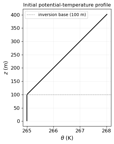
Initial conditions follow the GABLS1 protocol (Beare et al. 2006):

• \(u = U_g = 8\) m s\(^{-1}\), \(v = w = 0\) everywhere.

• \(\theta = 265\) K for \(z \le 100\) m; \(\theta = 265 + 0.01(z-100)\) K above.

• Small random perturbations below 50 m to trigger the turbulent cascade.

The run directory ships with a ready-to-use script ``CreateInputs_SBL_GABLS1.py`` that writes input/vel.ini (three-column ASCII: \(u\), \(v\), \(w\)) and input/TH.ini (one-column ASCII: potential temperature), both stored in Fortran column-major order.

Run it once before the first simulation:

cd /path/to/runs/128x128x128_LASDD_SM_DP
python CreateInputs_SBL_GABLS1.py

Expected output:

GABLS1 initial conditions written to .../input
  Grid: nx=128, ny=128, nz=128, dz=3.1496 m
  vel.ini shape: (2097152, 3)
  TH.ini  shape: (2097152,)
  TH range: 264.990 - 265.010 K

The initial temperature profile is plotted below for reference.

The temperature profile can be visualised to confirm the initial stratification:

# Reconstruct the deterministic part of the initial temperature profile
# (nz, l_z, dz loaded from Config.py in the cell above)
z_plot = np.array([(k + 0.5) * dz for k in range(nz)])

TH_profile = np.where(z_plot <= 100.0, 265.0, 265.0 + 0.01 * (z_plot - 100.0))

fig, ax = plt.subplots(figsize=(4, 5))
ax.plot(TH_profile, z_plot, 'k-', linewidth=1.8)
ax.axhline(100, color='gray', linestyle='--', linewidth=0.8, label='inversion base (100 m)')
ax.set_xlabel(r'$\theta$ (K)', fontsize=13)
ax.set_ylabel(r'$z$ (m)',      fontsize=13)
ax.set_title('Initial potential-temperature profile', fontsize=12)
ax.legend(fontsize=10)
ax.grid(alpha=0.3)
plt.tight_layout()
plt.show()

---

6. Step 3 — Create the Surface Boundary-Condition File

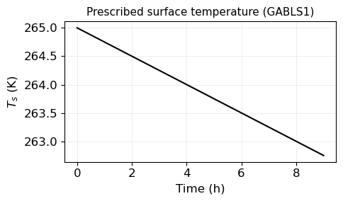
Because optSurfBC = 2, the solver reads the surface temperature at each time step from input/SurfaceBC.npz. The GABLS1 protocol prescribes a linear cooling rate of 0.25 K hr\(^{-1}\):

\[T_s(t) = 265 - 0.25 \cdot \frac{t}{3600}\]

Over 9 h the surface cools from 265 K to 262.75 K.

The run directory ships with ``CreateSurfaceBC_GABLS1.py``, which reads dt and SimTime directly from Config.py and writes the full time series to input/SurfaceBC.npz.

Run it once before the first simulation:

cd /path/to/runs/128x128x128_LASDD_SM_DP
python CreateSurfaceBC_GABLS1.py

Expected output:

Surface BC file written to .../input/SurfaceBC.npz
  Mode: linear cooling
  nsteps + 1    = 324001  (dt = 0.1 s, SimTime = 32400.0 s)
  T_s(t=0)      = 265.0000 K
  T_s(t=SimTime)= 262.7500 K
  T_s range     : [262.7500, 265.0000] K

The prescribed cooling curve is shown below.

# Prescribed surface temperature — GABLS1 linear cooling
# (dt_cfg, SimTime_cfg loaded from Config.py in the cell above)
nsteps   = int(np.ceil(SimTime_cfg / dt_cfg))
t_series = np.arange(0, nsteps + 1) * dt_cfg
T_sfc    = 265.0 - 0.25 * (t_series / 3600.0)

fig, ax = plt.subplots(figsize=(5, 3))
ax.plot(t_series / 3600, T_sfc, 'k-', linewidth=1.5)
ax.set_xlabel('Time (h)',   fontsize=12)
ax.set_ylabel(r'$T_s$ (K)', fontsize=12)
ax.set_title('Prescribed surface temperature (GABLS1)', fontsize=11)
ax.grid(alpha=0.3)
plt.tight_layout()
plt.show()

---

7. Step 4 — Launch the Solver

With Config.py, vel.ini, TH.ini, and SurfaceBC.npz in place, launch JAX-ALFA from the terminal:

export JAXALFA_RUNDIR=/path/to/128x128x128_LASDD_SM_DP
python /path/to/JAXALFA0.1/src/Main.py

The solver writes statistics to output/ALFA_Statistics_Iteration_*.npz every OutputInterval_sec seconds (60 s → one file per minute → 540 files for a 9-hour run).

Progress monitoring: the log file run.log (or stdout) prints a one-line summary every OutputInterval_sec seconds showing the current simulation time, wall-clock time per step, and the instantaneous friction velocity \(u_*\).

---

8. Step 5 - Load and Inspect the Output

Each statistics file contains horizontally averaged profiles sampled every SampleInterval_sec seconds (10 s) and time-averaged over OutputInterval_sec (60 s). The arrays stored in each .npz file are:

Array	Description	Grid
U, V, TH	Mean velocity components and potential temperature	half levels
u2, v2, w2	Resolved velocity variances	half / full levels
TH2	Resolved temperature variance	half levels
uv, uw, vw	Resolved momentum fluxes	half / full levels
txy, txz, tyz	SGS stress components	half / full levels
wTH	Resolved heat flux	full levels
qz	SGS heat flux	full levels

OutputDir = RunDir / 'output'


def get_stat_files(output_dir):
    """Return statistics files sorted by iteration number."""
    pattern = str(output_dir / 'ALFA_Statistics_Iteration_*.npz')
    files = sorted(
        glob.glob(pattern),
        key=lambda x: int(re.search(r'Iteration_(\d+)', x).group(1))
    )
    return files


stat_files = get_stat_files(OutputDir)
print(f'{len(stat_files)} statistics files found in {OutputDir}')

if not stat_files:
    raise FileNotFoundError(
        'No ALFA_Statistics_Iteration_*.npz files were found. Run the solver first, '
        'or point RunDir to a completed GABLS1 run.'
    )

with np.load(stat_files[0]) as d:
    print('Arrays in each file:', sorted(d.keys()))
    print('Profile length (nz):', d['U'].shape)

540 statistics files found in /Users/sukantabasu/Dropbox/Codes/LES/JAX-ALFA/JAXALFA0.1/examples/SBL_GABLS1/runs/128x128x128_LASDD_SM_DP/output
Arrays in each file: ['Beta1', 'Beta2', 'Cs2PrRatio', 'Cs2_1', 'Cs2_2', 'M_sfc', 'Q', 'Q2', 'TH', 'TH2', 'U', 'Ugal', 'V', 'W', 'ZeRo1D', 'dQdz', 'dTHdz', 'dUdz', 'dVdz', 'qHz', 'qm_sfc', 'qz', 'qz_sfc', 'txy', 'txz', 'tyz', 'u2', 'uTH', 'ustar', 'uv', 'uw', 'v2', 'vTH', 'vw', 'w2', 'wQ', 'wTH']
Profile length (nz): (128,)

8.1 Quasi-steady state averaging window

The GABLS1 benchmark defines the quasi-steady state as hours 8–9. We average over all statistics files in that window.

# (nz, l_z, OutputInterval_sec loaded from Config.py in the cell above)
T_start, T_end = 8 * 3600, 9 * 3600
i_start = int(T_start / OutputInterval_sec) - 1
i_end   = int(T_end   / OutputInterval_sec) - 1

# Vertical grids
z   = np.array([(k + 0.5) * l_z / (nz - 1) for k in range(nz)])   # half levels
z_w = np.array([k          * l_z / (nz - 1) for k in range(nz)])   # full levels

print(f'Averaging window: file indices {i_start}–{i_end} '
      f'({i_end - i_start + 1} files)')
print(f'Half-level range: {z[0]:.2f}–{z[-1]:.2f} m')

Averaging window: file indices 479–539 (61 files)
Half-level range: 1.57–401.57 m

def load_time_average(stat_files, i_start, i_end):
    """Load and time-average statistics over [i_start, i_end] inclusive."""
    if len(stat_files) <= i_end:
        raise ValueError(
            f'Need at least {i_end + 1} statistics files for the 8-9 h average; '
            f'found {len(stat_files)}.'
        )

    keys = ['U', 'V', 'TH', 'u2', 'v2', 'w2', 'TH2',
            'uv', 'uw', 'vw', 'txy', 'txz', 'tyz', 'wTH', 'qz']
    stacks = {k: [] for k in keys}

    for f in stat_files:
        with np.load(f) as d:
            missing = [k for k in keys if k not in d]
            if missing:
                raise KeyError(f'{f} is missing arrays: {missing}')
            for k in keys:
                stacks[k].append(d[k])

    sl = slice(i_start, i_end + 1)
    return {k: np.mean(np.array(stacks[k])[sl], axis=0) for k in keys}


avg = load_time_average(stat_files, i_start, i_end)

# Convenience: total (resolved + SGS) fluxes
uw_tot  = avg['uw']  + avg['txz']
vw_tot  = avg['vw']  + avg['tyz']
wTH_tot = avg['wTH'] + avg['qz']
S_mag   = np.sqrt(avg['U']**2 + avg['V']**2)

print('Time-averaged profiles loaded.')
print(f"  U range  : {avg['U'].min():.2f} - {avg['U'].max():.2f} m/s")
print(f"  TH range : {avg['TH'].min():.2f} - {avg['TH'].max():.2f} K")

Time-averaged profiles loaded.
  U range  : 1.62 - 9.46 m/s
  TH range : 263.19 - 268.02 K

---

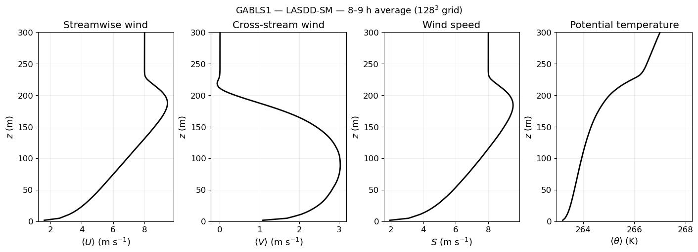
9. Mean Wind and Temperature Profiles

The panels below show the streamwise velocity \(U\), cross-stream velocity \(V\), wind-speed magnitude \(S\), and mean potential temperature \(\theta\) averaged over hours 8–9.

plt.rcParams.update({'font.size': 12, 'axes.labelsize': 13})

fig, axs = plt.subplots(1, 4, figsize=(14, 5), constrained_layout=True)

axs[0].plot(avg['U'], z, 'k-', linewidth=2)
axs[0].set_xlabel(r'$\langle U \rangle$ (m s$^{-1}$)')
axs[0].set_ylabel(r'$z$ (m)')
axs[0].set_title('Streamwise wind')

axs[1].plot(avg['V'], z, 'k-', linewidth=2)
axs[1].set_xlabel(r'$\langle V \rangle$ (m s$^{-1}$)')
axs[1].set_title('Cross-stream wind')

axs[2].plot(S_mag, z, 'k-', linewidth=2)
axs[2].set_xlabel(r'$S$ (m s$^{-1}$)')
axs[2].set_title('Wind speed')

axs[3].plot(avg['TH'], z, 'k-', linewidth=2)
axs[3].set_xlabel(r'$\langle \theta \rangle$ (K)')
axs[3].set_title('Potential temperature')

for ax in axs:
    ax.set_ylim(0, 300)
    ax.grid(alpha=0.3)
    ax.set_ylabel(r'$z$ (m)')

fig.suptitle('GABLS1 — LASDD-SM — 8–9 h average ($128^3$ grid)', fontsize=13)
plt.show()

---

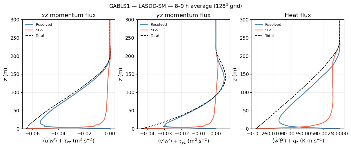
10. Momentum and Heat Fluxes

The total vertical flux is the sum of the resolved turbulent flux and the SGS contribution. In a well-resolved LES the SGS fraction should be small in the bulk and larger only near the surface.

fig, axs = plt.subplots(1, 3, figsize=(12, 5), constrained_layout=True)

# Total uw stress
axs[0].plot(avg['uw'],  z_w, color='steelblue', linewidth=2, label='Resolved')
axs[0].plot(avg['txz'], z_w, color='tomato',    linewidth=2, label='SGS')
axs[0].plot(uw_tot,     z_w, 'k--',             linewidth=1.5, label='Total')
axs[0].set_xlabel(r"$\langle u'w' \rangle + \tau_{xz}$ (m$^2$ s$^{-2}$)")
axs[0].set_title(r'$xz$ momentum flux')

# Total vw stress
axs[1].plot(avg['vw'],  z_w, color='steelblue', linewidth=2, label='Resolved')
axs[1].plot(avg['tyz'], z_w, color='tomato',    linewidth=2, label='SGS')
axs[1].plot(vw_tot,     z_w, 'k--',             linewidth=1.5, label='Total')
axs[1].set_xlabel(r"$\langle v'w' \rangle + \tau_{yz}$ (m$^2$ s$^{-2}$)")
axs[1].set_title(r'$yz$ momentum flux')

# Total heat flux
axs[2].plot(avg['wTH'], z_w, color='steelblue', linewidth=2, label='Resolved')
axs[2].plot(avg['qz'],  z_w, color='tomato',    linewidth=2, label='SGS')
axs[2].plot(wTH_tot,    z_w, 'k--',             linewidth=1.5, label='Total')
axs[2].set_xlabel(r"$\langle w'\theta' \rangle + q_z$ (K m s$^{-1}$)")
axs[2].set_title('Heat flux')

for ax in axs:
    ax.set_ylim(0, 300)
    ax.set_ylabel(r'$z$ (m)')
    ax.legend(fontsize=9, frameon=False)
    ax.grid(alpha=0.3)

fig.suptitle('GABLS1 — LASDD-SM — 8–9 h average ($128^3$ grid)', fontsize=13)
plt.show()

---

11. Temporal Evolution of the Friction Velocity

The friction velocity \(u_* = \bigl(-\langle u'w' \rangle_s\bigr)^{1/2}\) at the surface provides a compact diagnostic of the boundary-layer spin-up and quasi-steady approach. We compute it from the total surface stress (uw_tot[0], vw_tot[0]) as a function of time.

ustar_series = []
time_series  = []

for idx, f in enumerate(stat_files):
    with np.load(f) as d:
        uw_surf  = d['uw'][0]  + d['txz'][0]
        vw_surf  = d['vw'][0]  + d['tyz'][0]
        tau_surf = np.sqrt(uw_surf**2 + vw_surf**2)
        ustar_series.append(np.sqrt(tau_surf))
    time_series.append((idx + 1) * OutputInterval_sec / 3600.0)  # hours

ustar_series = np.array(ustar_series)
time_series  = np.array(time_series)

fig, ax = plt.subplots(figsize=(6, 3.5))
ax.plot(time_series, ustar_series, 'k-', linewidth=1.5)
ax.axvspan(8, 9, alpha=0.12, color='steelblue', label='Averaging window')
ax.set_xlabel('Time (h)', fontsize=12)
ax.set_ylabel(r'$u_*$ (m s$^{-1}$)', fontsize=12)
ax.set_title('GABLS1 - LASDD-SM - friction velocity', fontsize=11)
ax.legend(fontsize=10, frameon=False)
ax.grid(alpha=0.3)
plt.tight_layout()
plt.show()

window = (time_series >= 8) & (time_series <= 9)
ustar_avg = np.mean(ustar_series[window])
print(f'u* averaged over 8-9 h: {ustar_avg:.4f} m/s')

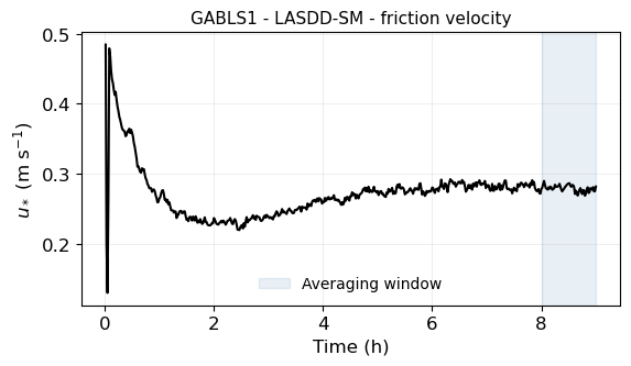
u* averaged over 8-9 h: 0.2788 m/s

---

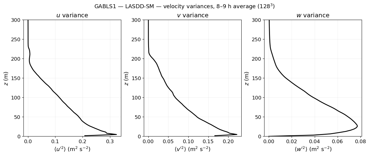
12. Velocity Variances

Resolved velocity variances characterise the turbulent intensity in each direction. Under stable stratification the vertical component \(\sigma_w^2\) is strongly suppressed compared to the horizontal components.

fig, axs = plt.subplots(1, 3, figsize=(12, 5), constrained_layout=True)

axs[0].plot(avg['u2'], z,   'k-', linewidth=2)
axs[0].set_xlabel(r"$\langle u'^2 \rangle$ (m$^2$ s$^{-2}$)")
axs[0].set_title(r'$u$ variance')

axs[1].plot(avg['v2'], z,   'k-', linewidth=2)
axs[1].set_xlabel(r"$\langle v'^2 \rangle$ (m$^2$ s$^{-2}$)")
axs[1].set_title(r'$v$ variance')

axs[2].plot(avg['w2'], z_w, 'k-', linewidth=2)
axs[2].set_xlabel(r"$\langle w'^2 \rangle$ (m$^2$ s$^{-2}$)")
axs[2].set_title(r'$w$ variance')

for ax in axs:
    ax.set_ylim(0, 300)
    ax.set_ylabel(r'$z$ (m)')
    ax.grid(alpha=0.3)

fig.suptitle('GABLS1 — LASDD-SM — velocity variances, 8–9 h average ($128^3$)', fontsize=13)
plt.show()

---

13. Next Steps

Now that you have a working GABLS1 run you can:

• Change the SGS model — edit optSgs in Config.py (1 = LASDD-SM, 2 = LASDD-WL, 3 = LAD-SM, 4 = LAD-WL) and re-run.

• Change precision — set use_double_precision = False for float32 and compare with the double-precision reference.

• Change resolution — adjust nx, ny, nz (and dt if needed for stability) to explore resolution sensitivity.

• Explore the Case Studies section for more complex examples (CBL, NBL, GABLS3, Wangara diurnal cycle).

See the API Reference section for a complete description of every module and configuration parameter.