GABLS1 LES Intercomparison Study for Stable Boundary Layers: SGS Model Coefficients
[1]:
from IPython.display import display, Markdown
from datetime import datetime, timezone
display(Markdown(f"*Last run: {datetime.now(timezone.utc).strftime('%B %d, %Y at %H:%M UTC')}*"))
Last run: June 24, 2026 at 09:27 UTC
For case setup and physical parameters, see the Description notebook.
Vertical profiles of the SGS coefficients — Smagorinsky coefficient \(C_s\), SGS Prandtl number \(\mathrm{Pr}_{SGS}\), and scale-dependence parameters \(\beta_1\) (momentum) and \(\beta_2\) (scalar) — are compared across the four grid resolutions (\(64^3\), \(128^3\), \(256^3\), \(384^3\)) for a user-selected SGS model. Averaging window: 8–9 h.
Setup
The next cells load Python packages, locate the simulation outputs, and define the grid and averaging window used throughout the notebook.
[12]:
import os
import re
import glob
import numpy as np
import matplotlib.pyplot as plt
from pathlib import Path
Output directories
[13]:
from pathlib import Path

# Base directory (jaxalfa/)
def find_repo_root(start=None):
    path = Path(start or ('__file__' in globals() and __file__) or Path.cwd()).resolve()
    for candidate in (path, *path.parents):
        if (candidate / 'examples').is_dir() and (candidate / 'docs').is_dir():
            return candidate
    raise FileNotFoundError('Could not locate jaxalfa repository root')

BaseDir = find_repo_root()

def read_config(run_dir):
    cfg = {}
    exec((run_dir / 'Config.py').read_text(), cfg)
    return cfg


optSGS = 1  # LASDD-SM: 1, LASDD-WL: 2, LAD-SM: 3, LAD-WL: 4, STAB-SM: 5

sgs_names = {1: 'LASDD-SM', 2: 'LASDD-WL', 3: 'LAD-SM', 4: 'LAD-WL', 5: 'STAB-SM'}

run_styles = {
    '64x64x64':          {'color': 'red',   'linestyle': '-'},
    '128x128x128':       {'color': 'blue',  'linestyle': '-'},
    '256x256x256':  {'color': 'green', 'linestyle': '-'},
    '384x384x384':       {'color': 'black', 'linestyle': '-'},
}

_sgs = {1: 'LASDD_SM', 2: 'LASDD_WL', 3: 'LAD_SM', 4: 'LAD_WL', 5: 'STABSM'}

# Precision is hardcoded per resolution for this case
OutputDir1 = BaseDir / f'examples/SBL_GABLS1/runs/64x64x64_{_sgs[optSGS]}_DP/output'
OutputDir2 = BaseDir / f'examples/SBL_GABLS1/runs/128x128x128_{_sgs[optSGS]}_DP/output'
OutputDir3 = BaseDir / f'examples/SBL_GABLS1/runs/256x256x256_{_sgs[optSGS]}_DP/output'
OutputDir4 = BaseDir / f'examples/SBL_GABLS1/runs/384x384x384_{_sgs[optSGS]}_SP/output'

# Note: STAB-SM (optSGS=5) reports Lambda_uvp2 as effective Cs^2; beta1=beta2=0 (no scale-dependence)
Case configuration
[14]:
cfg_1 = read_config(OutputDir1.parent)
cfg_2 = read_config(OutputDir2.parent)
cfg_3 = read_config(OutputDir3.parent)
cfg_4 = read_config(OutputDir4.parent)

nz_1 = int(cfg_1['nz'])
nz_2 = int(cfg_2['nz'])
nz_3 = int(cfg_3['nz'])
nz_4 = int(cfg_4['nz'])

l_z = float(cfg_1['l_z'])
z_damping = float(cfg_1.get('z_damping', np.nan))
OutputInterval_sec = float(cfg_1.get('OutputInterval_sec', 60.0))

# Averaging window — GABLS1 quasi-steady state (hours 8–9)
T_start = 8 * 3600   # s
T_end   = 9 * 3600   # s
Derived grid and averaging indices
[15]:
# Half levels — SGS coefficients live at UVP nodes
z_1 = np.array([(k + 0.5) * l_z / (nz_1 - 1) for k in range(nz_1)])
z_2 = np.array([(k + 0.5) * l_z / (nz_2 - 1) for k in range(nz_2)])
z_3 = np.array([(k + 0.5) * l_z / (nz_3 - 1) for k in range(nz_3)])
z_4 = np.array([(k + 0.5) * l_z / (nz_4 - 1) for k in range(nz_4)])

# File indices for the averaging window
T_start_index = int(T_start / OutputInterval_sec) - 1
T_end_index   = int(T_end   / OutputInterval_sec) - 1

print(f'Averaging window: file indices {T_start_index} – {T_end_index}')
Averaging window: file indices 479 – 539
SGS coefficient loader
[16]:
def LoadSGSAverage(stat_files, T_start_index, T_end_index, nz_expected):
    """Return time-averaged SGS coefficient profiles over the given window.

    Returns
    -------
    Cs2_1, Cs2_2 : ndarray (nz)
        Smagorinsky coefficient squared: (PlanarMean(Cs))^2 and PlanarMean(Cs^2).
    Cs2PrRatio : ndarray (nz)
        PlanarMean(Cs^2 / Pr_T) profile.
    Beta1, Beta2 : ndarray (nz)
        Scale-dependence parameters for momentum and scalar.
    """
    if len(stat_files) == 0:
        print(f'No statistics files available; plotting NaN placeholders for nz={nz_expected}.')
        nan = np.full(nz_expected, np.nan)
        return nan, nan.copy(), nan.copy(), nan.copy(), nan.copy()

    sl = slice(T_start_index, min(T_end_index + 1, len(stat_files)))
    if sl.start >= len(stat_files):
        print(f'Averaging window starts after available files; plotting NaN placeholders for nz={nz_expected}.')
        nan = np.full(nz_expected, np.nan)
        return nan, nan.copy(), nan.copy(), nan.copy(), nan.copy()

    Cs2_1_list = []; Cs2_2_list = []; Cs2PR_list = []
    B1_list    = []; B2_list    = []

    for f in stat_files[sl]:
        with np.load(f) as d:
            Cs2_1_list.append(d['Cs2_1'])
            Cs2_2_list.append(d['Cs2_2'])
            Cs2PR_list.append(d['Cs2PrRatio'])
            B1_list.append(d['Beta1'])
            B2_list.append(d['Beta2'])

    return (
        np.mean(Cs2_1_list, axis=0),
        np.mean(Cs2_2_list, axis=0),
        np.mean(Cs2PR_list, axis=0),
        np.mean(B1_list,    axis=0),
        np.mean(B2_list,    axis=0),
    )
Available statistics files
[17]:
def get_stat_files(output_dir):
    files = sorted(
        glob.glob(str(output_dir / 'ALFA_Statistics_Iteration_*.npz')),
        key=lambda x: int(re.search(r'Iteration_(\d+)', x).group(1))
    )
    return files

StatFiles1 = get_stat_files(OutputDir1)
StatFiles2 = get_stat_files(OutputDir2)
StatFiles3 = get_stat_files(OutputDir3)
StatFiles4 = get_stat_files(OutputDir4)

print(f'64^3        : {len(StatFiles1)} files')
print(f'128^3       : {len(StatFiles2)} files')
print(f'256^3       : {len(StatFiles3)} files')
print(f'384^3       : {len(StatFiles4)} files')
64^3        : 540 files
128^3       : 540 files
256^3       : 540 files
384^3       : 540 files
Temporally averaged profiles
[18]:
(Cs2_1_avg_1, Cs2_2_avg_1, Cs2PR_avg_1, B1_avg_1, B2_avg_1) = \
    LoadSGSAverage(StatFiles1, T_start_index, T_end_index, nz_1)

(Cs2_1_avg_2, Cs2_2_avg_2, Cs2PR_avg_2, B1_avg_2, B2_avg_2) = \
    LoadSGSAverage(StatFiles2, T_start_index, T_end_index, nz_2)

(Cs2_1_avg_3, Cs2_2_avg_3, Cs2PR_avg_3, B1_avg_3, B2_avg_3) = \
    LoadSGSAverage(StatFiles3, T_start_index, T_end_index, nz_3)

(Cs2_1_avg_4, Cs2_2_avg_4, Cs2PR_avg_4, B1_avg_4, B2_avg_4) = \
    LoadSGSAverage(StatFiles4, T_start_index, T_end_index, nz_4)

# SGS coefficient: two averaging conventions
# Method 1: C = PlanarMean(C), then squared for storage → take sqrt
# Method 2: C = sqrt(PlanarMean(C^2))
Cs_m1_1 = np.sqrt(np.abs(Cs2_1_avg_1));  Cs_m2_1 = np.sqrt(np.abs(Cs2_2_avg_1))
Cs_m1_2 = np.sqrt(np.abs(Cs2_1_avg_2));  Cs_m2_2 = np.sqrt(np.abs(Cs2_2_avg_2))
Cs_m1_3 = np.sqrt(np.abs(Cs2_1_avg_3));  Cs_m2_3 = np.sqrt(np.abs(Cs2_2_avg_3))
Cs_m1_4 = np.sqrt(np.abs(Cs2_1_avg_4));  Cs_m2_4 = np.sqrt(np.abs(Cs2_2_avg_4))

# PrSGS = Cs2_2 / Cs2PrRatio  (NaN where Cs2PrRatio ≈ 0)
_tol = 1e-10
PrSGS_1 = np.where(Cs2PR_avg_1 > _tol, Cs2_2_avg_1 / Cs2PR_avg_1, np.nan)
PrSGS_2 = np.where(Cs2PR_avg_2 > _tol, Cs2_2_avg_2 / Cs2PR_avg_2, np.nan)
PrSGS_3 = np.where(Cs2PR_avg_3 > _tol, Cs2_2_avg_3 / Cs2PR_avg_3, np.nan)
PrSGS_4 = np.where(Cs2PR_avg_4 > _tol, Cs2_2_avg_4 / Cs2PR_avg_4, np.nan)

print(f'Averaging over {T_end_index - T_start_index + 1} files '
      f'({T_start/3600:.1f}–1{T_end/3600:.1f} h)')
Averaging over 61 files (8.0–19.0 h)
/var/folders/fm/088xfr2x1vs0yr7dmrdgjfrh0000gn/T/ipykernel_34151/2150077097.py:26: RuntimeWarning: invalid value encountered in divide
  PrSGS_4 = np.where(Cs2PR_avg_4 > _tol, Cs2_2_avg_4 / Cs2PR_avg_4, np.nan)
[19]:
plt.rcParams.update({
    "text.usetex": True,
    "font.size": 14,
    "axes.labelsize": 16,
    "xtick.labelsize": 12,
    "ytick.labelsize": 12
})
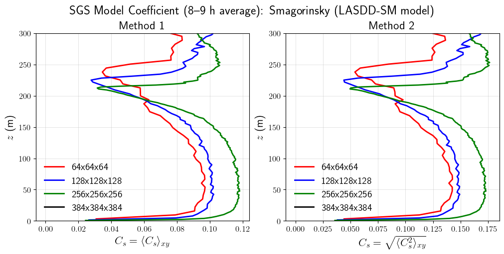
SGS Model Coefficient
For SM variants (LASDD-SM, LAD-SM) the coefficient is the Smagorinsky coefficient \(C_s\); for WL variants (LASDD-WL, LAD-WL) it is the Wong-Lilly SGS coefficient \(C\). Two planar-averaging conventions are shown:
Method 1 (left): \(C = \langle C \rangle_{xy}\) — planar mean of the pointwise field.
Method 2 (right): \(C = \sqrt{\langle C^2 \rangle_{xy}}\) — root of the planar mean of \(C^2\).
By Jensen’s inequality, Method 2 \(\geq\) Method 1.
[20]:
fig, axs = plt.subplots(1, 2, figsize=(10, 5), constrained_layout=True)

_coeff_sym  = r'C_s' if optSGS in [1, 3] else r'C'
_coeff_name = 'Smagorinsky' if optSGS in [1, 3] else 'Wong-Lilly SGS'

for lbl, Cs_m1, Cs_m2, z in [
    ('64x64x64', Cs_m1_1, Cs_m2_1, z_1),
    ('128x128x128', Cs_m1_2, Cs_m2_2, z_2),
    ('256x256x256', Cs_m1_3, Cs_m2_3, z_3),
    ('384x384x384', Cs_m1_4, Cs_m2_4, z_4),
]:
    style = run_styles[lbl]
    axs[0].plot(Cs_m1, z, color=style['color'], linestyle=style['linestyle'], linewidth=2, label=lbl)
    axs[1].plot(Cs_m2, z, color=style['color'], linestyle=style['linestyle'], linewidth=2, label=lbl)

axs[0].set_xlabel(rf"${_coeff_sym} = \langle {_coeff_sym} \rangle_{{xy}}$")
axs[0].set_ylabel(r"$z$ (m)")
axs[0].set_title("Method 1")

axs[1].set_xlabel(rf"${_coeff_sym} = \sqrt{{\langle {_coeff_sym}^2 \rangle_{{xy}}}}$")
axs[1].set_ylabel(r"$z$ (m)")
axs[1].set_title("Method 2")

for ax in axs:
    ax.set_ylim(0, z_damping)
    ax.grid()
    ax.legend(frameon=False)

fig.suptitle(f"SGS Model Coefficient (8--9 h average): {_coeff_name} ({sgs_names[optSGS]} model)", fontsize=18)
plt.show()
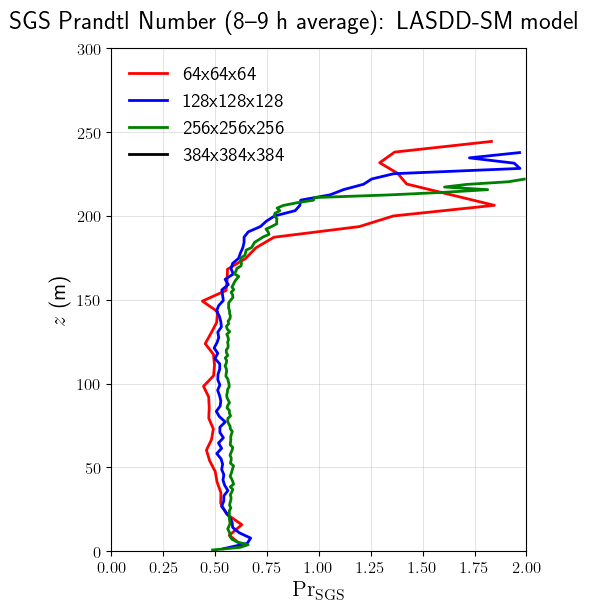
SGS Prandtl Number
The SGS Prandtl number is derived from the stored \(\langle C^2 \rangle_{xy}\) and \(\langle C^2/\mathrm{Pr}_\mathrm{SGS} \rangle_{xy}\) profiles:
where \(\langle C^2 \rangle_{xy}\) is Method 2 (root-mean-square planar average). Both numerator and denominator are planar means of pointwise 3D fields, making their ratio consistent. Points where \(\langle C^2/\mathrm{Pr}_\mathrm{SGS} \rangle_{xy} < 10^{-10}\) or \(\mathrm{Pr}_\mathrm{SGS} > \mathrm{Pr}_{\mathrm{SGS},\mathrm{max}}\) are masked.
[21]:
fig, ax = plt.subplots(figsize=(5, 6), constrained_layout=True)

PrSGS_xlim = 2.0  # adjust if needed

for lbl, PrSGS, z in [
    ('64x64x64', PrSGS_1, z_1),
    ('128x128x128', PrSGS_2, z_2),
    ('256x256x256', PrSGS_3, z_3),
    ('384x384x384', PrSGS_4, z_4),
]:
    style = run_styles[lbl]
    mask = (z <= z_damping) & (PrSGS <= PrSGS_xlim)
    ax.plot(PrSGS[mask], z[mask], color=style['color'], linestyle=style['linestyle'], linewidth=2, label=lbl)

ax.set_xlabel(r"$\mathrm{Pr}_\mathrm{SGS}$")
ax.set_ylabel(r"$z$ (m)")
ax.set_xlim(0, PrSGS_xlim)
ax.set_ylim(0, z_damping)
ax.grid()
ax.legend(frameon=False)

fig.suptitle(f"SGS Prandtl Number (8--9 h average): {sgs_names[optSGS]} model", fontsize=18)
plt.show()
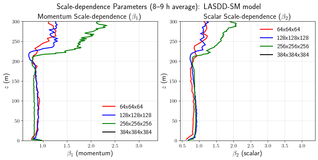
Scale-dependence Parameters
The scale-dependence parameters \(\beta_1\) (momentum) and \(\beta_2\) (scalar) characterize how the dynamic coefficient varies across filter scales. Values near unity indicate weak scale dependence; departures signal the model adapting to local turbulence structure.
[22]:
fig, axs = plt.subplots(1, 2, figsize=(10, 5), constrained_layout=True)

for lbl, B1, B2, z in [
    ('64x64x64',         B1_avg_1, B2_avg_1, z_1),
    ('128x128x128',      B1_avg_2, B2_avg_2, z_2),
    ('256x256x256', B1_avg_3, B2_avg_3, z_3),
    ('384x384x384',      B1_avg_4, B2_avg_4, z_4),
]:
    style = run_styles[lbl]
    axs[0].plot(B1, z, color=style['color'], linestyle=style['linestyle'], linewidth=2, label=lbl)
    axs[1].plot(B2, z, color=style['color'], linestyle=style['linestyle'], linewidth=2, label=lbl)

axs[0].set_xlabel(r"$\beta_1$ (momentum)")
axs[0].set_ylabel(r"$z$ (m)")
axs[0].set_title(r"Momentum Scale-dependence ($\beta_1$)")

axs[1].set_xlabel(r"$\beta_2$ (scalar)")
axs[1].set_ylabel(r"$z$ (m)")
axs[1].set_title(r"Scalar Scale-dependence ($\beta_2$)")

for ax in axs:
    ax.set_ylim(0, z_damping)
    ax.grid()
    ax.legend(frameon=False)

fig.suptitle(f"Scale-dependence Parameters (8--9 h average): {sgs_names[optSGS]} model", fontsize=18)
plt.show()