GABLS4 LES Intercomparison Study for Stable Boundary Layers: Sensitivity with respect to Numerical Precision
[1]:
from IPython.display import display, Markdown
from datetime import datetime, timezone
display(Markdown(f"*Last run: {datetime.now(timezone.utc).strftime('%B %d, %Y at %H:%M UTC')}*"))
Last run: June 24, 2026 at 09:27 UTC
For case setup and physical parameters, see the Description notebook.
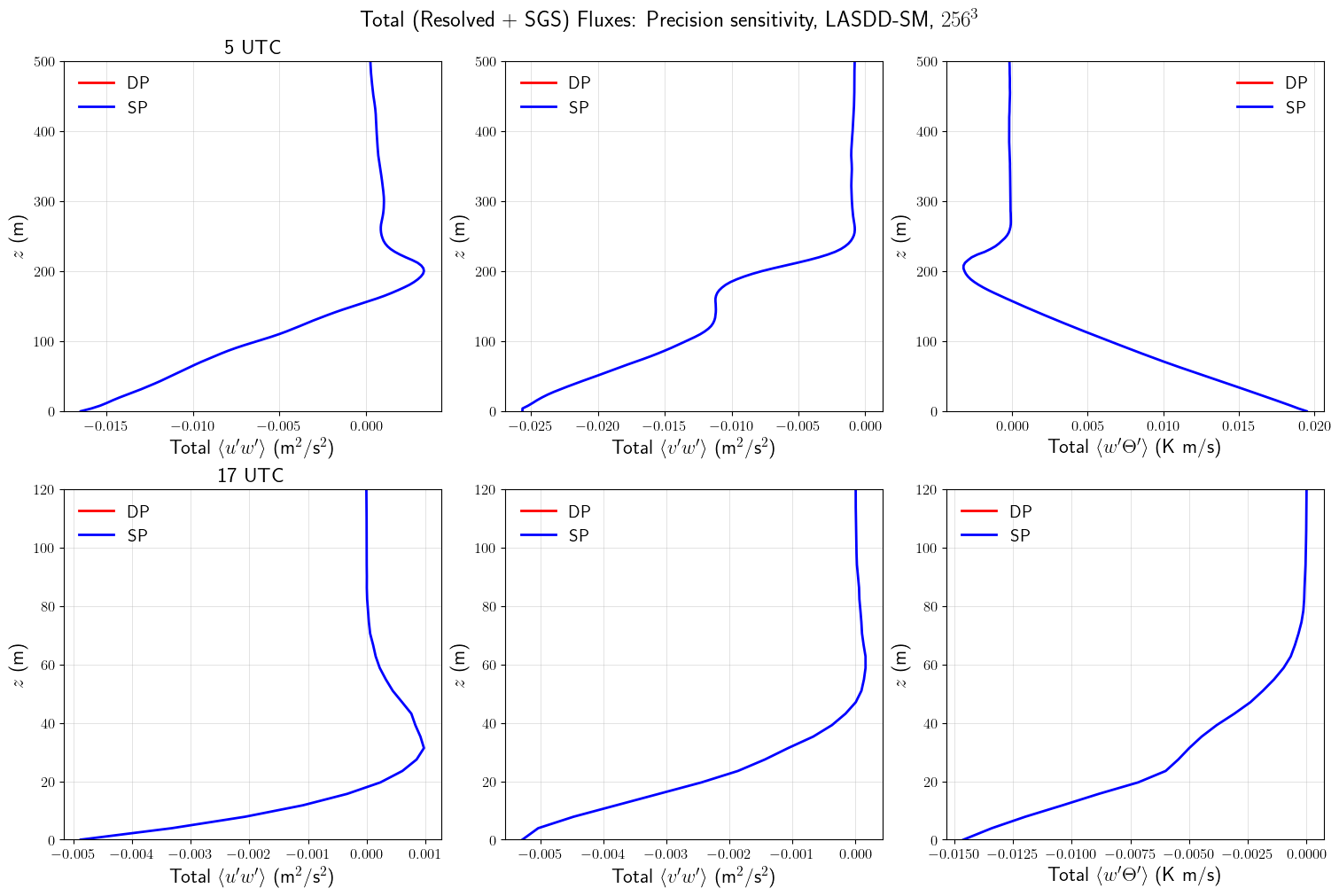
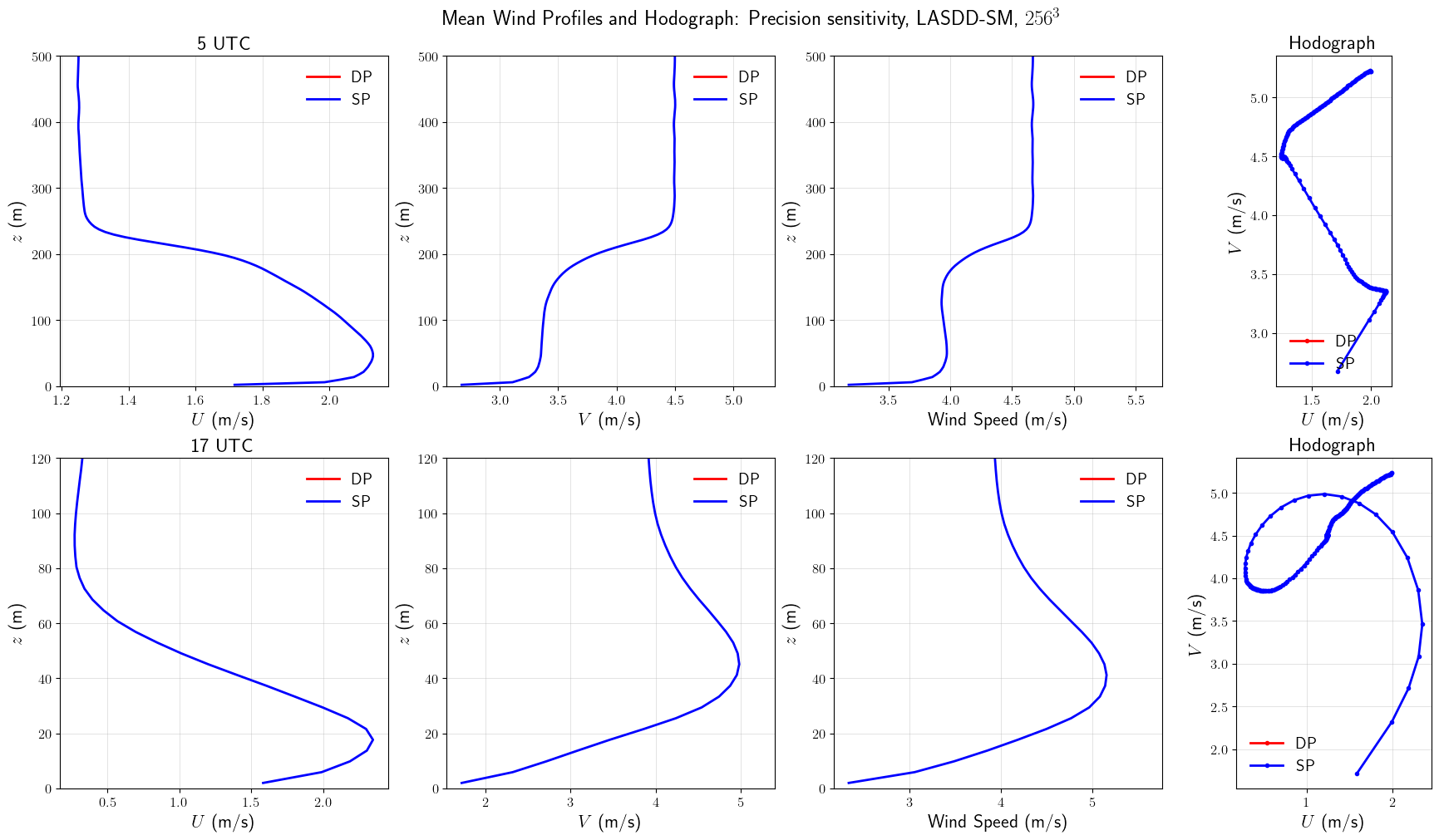
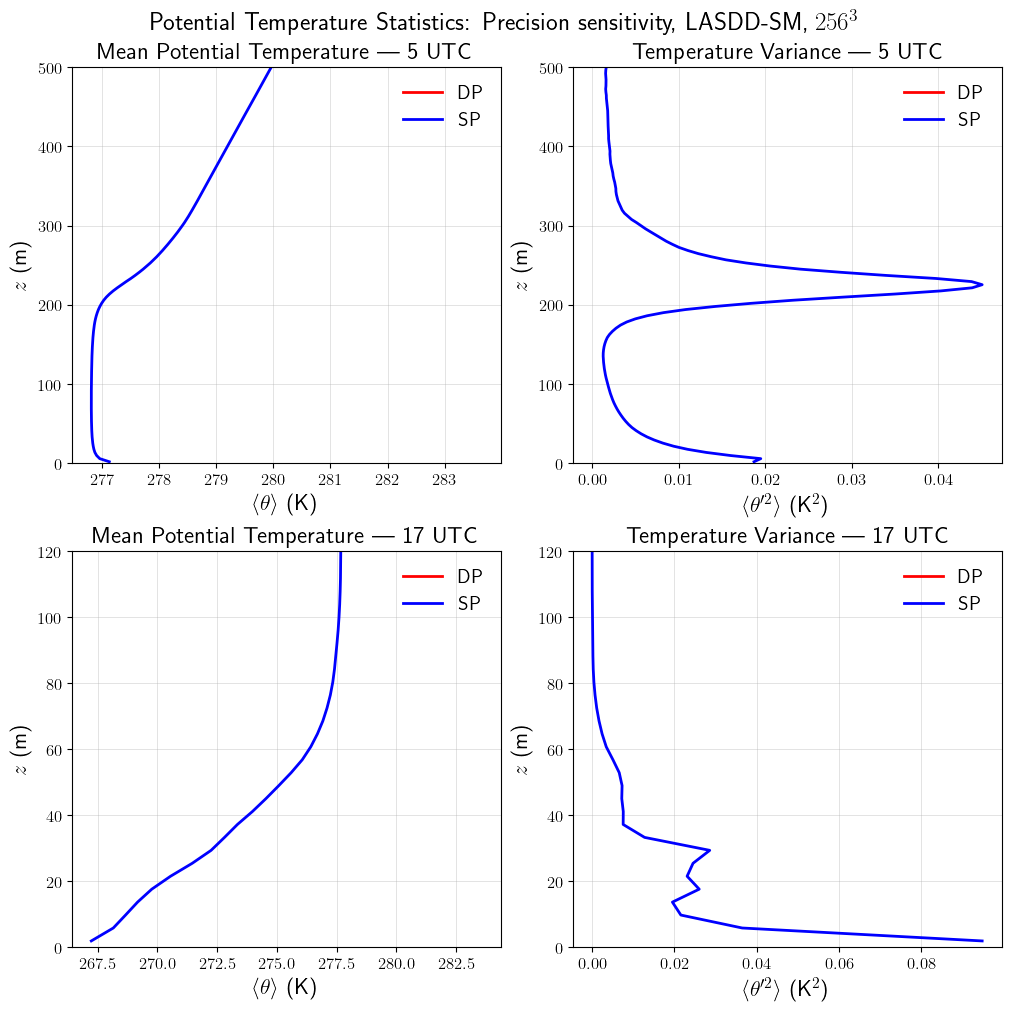
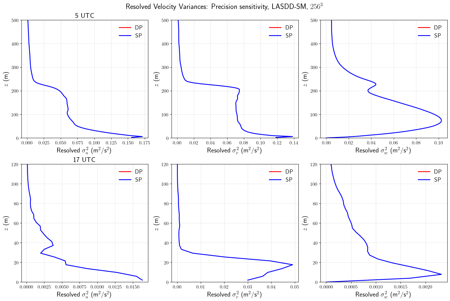
Precisions compared: double (DP), single (SP); SGS: LASDD-SM, grid: \(256^3\). Profiles shown at 5 UTC (simulation hour 5) and 17 UTC (simulation hour 17). The simulation starts at 0 UTC; the Dome C site is at 75.1°S.
Setup
The next cells load Python packages, locate the simulation outputs, and define the vertical grid and snapshot times.
[1]:
import os
import re
import glob
import numpy as np
import matplotlib.pyplot as plt
from pathlib import Path
Output directories
[2]:
from pathlib import Path

def find_repo_root(start=None):
    path = Path(start or ('__file__' in globals() and __file__) or Path.cwd()).resolve()
    for candidate in (path, *path.parents):
        if (candidate / 'examples').is_dir() and (candidate / 'docs').is_dir():
            return candidate
    raise FileNotFoundError('Could not locate jaxalfa repository root')

BaseDir = find_repo_root()

def read_config(run_dir):
    cfg = {}
    exec((run_dir / 'Config.py').read_text(), cfg)
    return cfg


optSGS = 1   # LASDD-SM: 1, LASDD-WL: 2, LAD-SM: 3, LAD-WL: 4
optRes = 3   # 64x64x64: 1, 128x128x128: 2, 256x256x256: 3, 384x384x384: 4

_res       = {1: '64x64x64', 2: '128x128x128', 3: '256x256x256', 4: '384x384x384'}
_sgs       = {1: 'LASDD_SM', 2: 'LASDD_WL',   3: 'LAD_SM',      4: 'LAD_WL'}
_sgs_label = {1: 'LASDD-SM', 2: 'LASDD-WL',   3: 'LAD-SM',      4: 'LAD-WL'}
_res_label = {1: r'$64^3$',  2: r'$128^3$',   3: r'$256^3$',    4: r'$384^3$'}

_run = f"{_res[optRes]}_{_sgs[optSGS]}"

OutputDir_DP = BaseDir / f'examples_A6000ada/SBL_GABLS4/runs/{_run}_DP/output'
OutputDir_SP = BaseDir / f'examples_A6000ada/SBL_GABLS4/runs/{_run}_SP/output'
Case configuration
[3]:
_cfg_ref = read_config(
    OutputDir_SP.parent if (OutputDir_SP.parent / 'Config.py').exists()
    else OutputDir_DP.parent
)

nz                 = int(_cfg_ref['nz'])
l_z                = float(_cfg_ref['l_z'])
OutputInterval_sec = float(_cfg_ref['OutputInterval_sec'])
z_damping          = float(_cfg_ref.get('z_damping', 700.0))

print(f'nz={nz}, l_z={l_z:g} m, OutputInterval={OutputInterval_sec:g} s')
print(f'Damping layer above z={z_damping:g} m')
nz=256, l_z=1000 m, OutputInterval=600 s
Damping layer above z=700 m
Vertical grid and snapshot indices
[4]:
# Half levels — U, V, TH, u2, v2, TH2
z   = np.array([(k + 0.5) * l_z / (nz - 1) for k in range(nz)])

# Full (staggered) levels — w, uw, vw, wTH, txz, tyz, qz
z_w = np.array([k * l_z / (nz - 1) for k in range(nz)])

# GABLS4 simulation starts at 0 UTC.
# 5 UTC  = simulation hour  5 h = 18 000 s
# 17 UTC = simulation hour 17 h = 61 200 s
T_snap1_s =  5.0 * 3600
T_snap2_s = 17.0 * 3600

snap1_index = int(T_snap1_s / OutputInterval_sec) - 1   # 29
snap2_index = int(T_snap2_s / OutputInterval_sec) - 1   # 101

print(f'5 UTC  (sim h  5): file index {snap1_index}')
print(f'17 UTC (sim h 17): file index {snap2_index}')
5 UTC  (sim h  5): file index 29
17 UTC (sim h 17): file index 101
Snapshot loader
[5]:
def LoadSnapshot(stat_files, snap_index, nz_expected):
    if len(stat_files) == 0 or snap_index >= len(stat_files):
        print(f'No data at index {snap_index}; plotting NaN placeholders for nz={nz_expected}.')
        nan = np.full(nz_expected, np.nan)
        return tuple(nan.copy() for _ in range(15))
    with np.load(stat_files[snap_index]) as d:
        return (
            d['U'].copy(),   d['V'].copy(),   d['TH'].copy(),
            d['u2'].copy(),  d['v2'].copy(),  d['w2'].copy(),
            d['TH2'].copy(),
            d['uv'].copy(),  d['uw'].copy(),  d['vw'].copy(),
            d['txy'].copy(), d['txz'].copy(), d['tyz'].copy(),
            d['wTH'].copy(), d['qz'].copy()
        )
Available statistics files
[6]:
def get_stat_files(output_dir):
    files = sorted(
        glob.glob(str(output_dir / 'ALFA_Statistics_Iteration_*.npz')),
        key=lambda x: int(re.search(r'Iteration_(\d+)', x).group(1))
    )
    return files

StatFiles_DP = get_stat_files(OutputDir_DP)
StatFiles_SP = get_stat_files(OutputDir_SP)

print(f'DP : {len(StatFiles_DP)} files')
print(f'SP : {len(StatFiles_SP)} files')
DP : 0 files
SP : 144 files
Load snapshots
[7]:
# ---- 5 UTC (simulation hour 5) ----
(U_DP_a, V_DP_a, TH_DP_a, u2_DP_a, v2_DP_a, w2_DP_a, TH2_DP_a,
 uv_DP_a, uw_DP_a, vw_DP_a, txy_DP_a, txz_DP_a, tyz_DP_a,
 wTH_DP_a, qz_DP_a) = LoadSnapshot(StatFiles_DP, snap1_index, nz)

(U_SP_a, V_SP_a, TH_SP_a, u2_SP_a, v2_SP_a, w2_SP_a, TH2_SP_a,
 uv_SP_a, uw_SP_a, vw_SP_a, txy_SP_a, txz_SP_a, tyz_SP_a,
 wTH_SP_a, qz_SP_a) = LoadSnapshot(StatFiles_SP, snap1_index, nz)

# ---- 17 UTC (simulation hour 17) ----
(U_DP_b, V_DP_b, TH_DP_b, u2_DP_b, v2_DP_b, w2_DP_b, TH2_DP_b,
 uv_DP_b, uw_DP_b, vw_DP_b, txy_DP_b, txz_DP_b, tyz_DP_b,
 wTH_DP_b, qz_DP_b) = LoadSnapshot(StatFiles_DP, snap2_index, nz)

(U_SP_b, V_SP_b, TH_SP_b, u2_SP_b, v2_SP_b, w2_SP_b, TH2_SP_b,
 uv_SP_b, uw_SP_b, vw_SP_b, txy_SP_b, txz_SP_b, tyz_SP_b,
 wTH_SP_b, qz_SP_b) = LoadSnapshot(StatFiles_SP, snap2_index, nz)

# ---- Derived quantities ----
S_DP_a = np.sqrt(U_DP_a**2 + V_DP_a**2);  S_DP_b = np.sqrt(U_DP_b**2 + V_DP_b**2)
S_SP_a = np.sqrt(U_SP_a**2 + V_SP_a**2);  S_SP_b = np.sqrt(U_SP_b**2 + V_SP_b**2)

uw_tot_DP_a = uw_DP_a + txz_DP_a;  uw_tot_DP_b = uw_DP_b + txz_DP_b
vw_tot_DP_a = vw_DP_a + tyz_DP_a;  vw_tot_DP_b = vw_DP_b + tyz_DP_b
wT_tot_DP_a = wTH_DP_a + qz_DP_a;  wT_tot_DP_b = wTH_DP_b + qz_DP_b

uw_tot_SP_a = uw_SP_a + txz_SP_a;  uw_tot_SP_b = uw_SP_b + txz_SP_b
vw_tot_SP_a = vw_SP_a + tyz_SP_a;  vw_tot_SP_b = vw_SP_b + tyz_SP_b
wT_tot_SP_a = wTH_SP_a + qz_SP_a;  wT_tot_SP_b = wTH_SP_b + qz_SP_b

print('Snapshots loaded.')
No data at index 29; plotting NaN placeholders for nz=256.
No data at index 101; plotting NaN placeholders for nz=256.
Snapshots loaded.
[8]:
plt.rcParams.update({
    'text.usetex'    : True,
    'font.size'      : 14,
    'axes.labelsize' : 16,
    'xtick.labelsize': 12,
    'ytick.labelsize': 12,
})

z_max = z_damping   # show only below the damping layer
z_max_a = 500.0     # 5 UTC profiles
z_max_b = 120.0     # 17 UTC profiles
z_maxs  = [z_max_a, z_max_b]

run_styles = {
    'DP': {'color': 'red',  'linestyle': '-'},
    'SP': {'color': 'blue', 'linestyle': '-'},
}

def prf(ax, x, z, xlabel, run_label):
    s = run_styles[run_label]
    ax.plot(x, z, color=s['color'], linestyle=s['linestyle'], linewidth=2, label=run_label)
    ax.set_xlabel(xlabel)
    ax.set_ylabel(r'$z$ (m)')
    ax.set_ylim(0, z_max)
Mean Wind and Hodograph
Horizontal mean wind components (\(U\), \(V\)), wind-speed magnitude, and hodograph at the two target times. Top row: 5 UTC (simulation hour 5); bottom row: 17 UTC (simulation hour 17).
[9]:
fig, axs = plt.subplots(2, 4, figsize=(18, 10), constrained_layout=True)

for row, (tag,
          U_DP,V_DP,S_DP, U_SP,V_SP,S_SP) in enumerate([
    ('5 UTC',  U_DP_a,V_DP_a,S_DP_a, U_SP_a,V_SP_a,S_SP_a),
    ('17 UTC', U_DP_b,V_DP_b,S_DP_b, U_SP_b,V_SP_b,S_SP_b),
]):
    z_max = z_maxs[row]
    prf(axs[row,0], U_DP, z, r'$U$ (m/s)',        'DP')
    prf(axs[row,0], U_SP, z, r'$U$ (m/s)',        'SP')
    prf(axs[row,1], V_DP, z, r'$V$ (m/s)',        'DP')
    prf(axs[row,1], V_SP, z, r'$V$ (m/s)',        'SP')
    prf(axs[row,2], S_DP, z, r'Wind Speed (m/s)', 'DP')
    prf(axs[row,2], S_SP, z, r'Wind Speed (m/s)', 'SP')

    axs[row,3].plot(U_DP, V_DP, color='red',  linestyle='-', marker='o',
                    linewidth=2, markersize=3, label='DP')
    axs[row,3].plot(U_SP, V_SP, color='blue', linestyle='-', marker='o',
                    linewidth=2, markersize=3, label='SP')
    axs[row,3].set_xlabel(r'$U$ (m/s)')
    axs[row,3].set_ylabel(r'$V$ (m/s)')
    axs[row,3].set_title('Hodograph')
    axs[row,3].set_aspect('equal')

    for ax in axs[row]:
        ax.grid(); ax.legend(frameon=False)
    axs[row,0].set_title(tag)

fig.suptitle(
    f'Mean Wind Profiles and Hodograph: Precision sensitivity, '
    f'{_sgs_label[optSGS]}, {_res_label[optRes]}',
    fontsize=18
)
plt.show()
Mean Potential Temperature and Temperature Variance
Horizontally averaged potential-temperature profile and resolved temperature variance. Top: 5 UTC; bottom: 17 UTC.
[10]:
fig, axs = plt.subplots(2, 2, figsize=(10, 10), constrained_layout=True)

for row, (tag,
          TH_DP,TH_SP, TH2_DP,TH2_SP) in enumerate([
    ('5 UTC',  TH_DP_a,TH_SP_a, TH2_DP_a,TH2_SP_a),
    ('17 UTC', TH_DP_b,TH_SP_b, TH2_DP_b,TH2_SP_b),
]):
    z_max = z_maxs[row]
    prf(axs[row,0], TH_DP,  z, r'$\langle\theta\rangle$ (K)',       'DP')
    prf(axs[row,0], TH_SP,  z, r'$\langle\theta\rangle$ (K)',       'SP')
    prf(axs[row,1], TH2_DP, z, r"$\langle\theta'^2\rangle$ (K$^2$)", 'DP')
    prf(axs[row,1], TH2_SP, z, r"$\langle\theta'^2\rangle$ (K$^2$)", 'SP')

    axs[row,0].set_title(f'Mean Potential Temperature — {tag}')
    axs[row,1].set_title(f'Temperature Variance — {tag}')
    for ax in axs[row]:
        ax.grid(); ax.legend(frameon=False)

fig.suptitle(
    f'Potential Temperature Statistics: Precision sensitivity, '
    f'{_sgs_label[optSGS]}, {_res_label[optRes]}',
    fontsize=18
)
plt.show()
Resolved Velocity Variances
Resolved variance profiles of \(u\), \(v\), and \(w\). Top: 5 UTC; bottom: 17 UTC.
[11]:
fig, axs = plt.subplots(2, 3, figsize=(15, 10), constrained_layout=True)

for row, (tag,
          u2_DP,v2_DP,w2_DP,
          u2_SP,v2_SP,w2_SP) in enumerate([
    ('5 UTC',  u2_DP_a,v2_DP_a,w2_DP_a, u2_SP_a,v2_SP_a,w2_SP_a),
    ('17 UTC', u2_DP_b,v2_DP_b,w2_DP_b, u2_SP_b,v2_SP_b,w2_SP_b),
]):
    z_max = z_maxs[row]
    prf(axs[row,0], u2_DP, z,   r'Resolved $\sigma_u^2$ (m$^2$/s$^2$)', 'DP')
    prf(axs[row,0], u2_SP, z,   r'Resolved $\sigma_u^2$ (m$^2$/s$^2$)', 'SP')
    prf(axs[row,1], v2_DP, z,   r'Resolved $\sigma_v^2$ (m$^2$/s$^2$)', 'DP')
    prf(axs[row,1], v2_SP, z,   r'Resolved $\sigma_v^2$ (m$^2$/s$^2$)', 'SP')
    prf(axs[row,2], w2_DP, z_w, r'Resolved $\sigma_w^2$ (m$^2$/s$^2$)', 'DP')
    prf(axs[row,2], w2_SP, z_w, r'Resolved $\sigma_w^2$ (m$^2$/s$^2$)', 'SP')

    for ax in axs[row]:
        ax.grid(); ax.legend(frameon=False)
    axs[row,0].set_title(tag)

fig.suptitle(
    f'Resolved Velocity Variances: Precision sensitivity, '
    f'{_sgs_label[optSGS]}, {_res_label[optRes]}',
    fontsize=18
)
plt.show()
Total Momentum and Heat Fluxes
Total (resolved + SGS) momentum and sensible heat fluxes. Top: 5 UTC; bottom: 17 UTC.
[12]:
fig, axs = plt.subplots(2, 3, figsize=(15, 10), constrained_layout=True)

for row, (tag,
          uw_DP,vw_DP,wt_DP,
          uw_SP,vw_SP,wt_SP) in enumerate([
    ('5 UTC',  uw_tot_DP_a,vw_tot_DP_a,wT_tot_DP_a,
               uw_tot_SP_a,vw_tot_SP_a,wT_tot_SP_a),
    ('17 UTC', uw_tot_DP_b,vw_tot_DP_b,wT_tot_DP_b,
               uw_tot_SP_b,vw_tot_SP_b,wT_tot_SP_b),
]):
    z_max = z_maxs[row]
    prf(axs[row,0], uw_DP, z_w, r"Total $\langle u'w'\rangle$ (m$^2$/s$^2$)", 'DP')
    prf(axs[row,0], uw_SP, z_w, r"Total $\langle u'w'\rangle$ (m$^2$/s$^2$)", 'SP')
    prf(axs[row,1], vw_DP, z_w, r"Total $\langle v'w'\rangle$ (m$^2$/s$^2$)", 'DP')
    prf(axs[row,1], vw_SP, z_w, r"Total $\langle v'w'\rangle$ (m$^2$/s$^2$)", 'SP')
    prf(axs[row,2], wt_DP, z_w, r"Total $\langle w'\Theta'\rangle$ (K m/s)",  'DP')
    prf(axs[row,2], wt_SP, z_w, r"Total $\langle w'\Theta'\rangle$ (K m/s)",  'SP')

    for ax in axs[row]:
        ax.grid(); ax.legend(frameon=False)
    axs[row,0].set_title(tag)

fig.suptitle(
    f'Total (Resolved + SGS) Fluxes: Precision sensitivity, '
    f'{_sgs_label[optSGS]}, {_res_label[optRes]}',
    fontsize=18
)
plt.show()